Excel Methodical manual. Good books on Excel and VBA
Master Excel easy! If you adhere to the opposite opinion, you did not come across a class allowance for learning the program.
I once had enough for all textbooks in a row. Swallow information in the hope of even slightly tighten the knowledge of Excel. To admit, went over dozens of books. And I realized that only units were coping with their task.
So, here is my distinguished list of the top 10 books on Excel:
1. John Waolenbach "Microsoft Excel 2013. User Bible"
2. John Waolenbach "Formulas in Microsoft Excel 2013"
|
|
Do you know what I regretted after buying this book? That she did not get into my hands much earlier. This is a real wisdom store! John Waolenbach by the hand will hold you from the elementary features of Excel before the workshop holds functions. You will learn how to work with cells and ranges, stroke with huge data arrays and extract the necessary information from them, process and analyze any type of data, and much more. The end will become such a cool special, that you can create custom functions in VBA yourself. Take and study "Formulas in Microsoft Excel 2013" from crust to crust. It is worth it! |

3. John Waolenbach "Excel 2013. Professional programming on VBA"
4. Bill Jelen and Michael Alexander "Summary Tables in Microsoft Excel"
|
|
Who do not want to raise the performance of work? Some reducing time costs for boring reports? Almost instantly evaluate and analyze data? What about cutting a long confusing report to a laconic and understandable? Complicated? Not at all! With consolidated tables in Microsoft Excel, all these tricks are easier than a paired turnip. If you often have to deal with complicated reporting, Bill Gelen's work and Michael Alexander - Must Have in your library. |

5. Curtis Fry "Microsoft Excel 2013. Step by step"
6. Greg Harvey "Microsoft Excel 2013 for Doodles"
7. Conrad Carlberg Business Analysis Using Excel
|
|
What can be more boring than tights with tons of reports? Sit and analyze the situation or deal with business tasks accounting for hours. Yes drop! You are seriously not aware that all this can be easily done in Excel? This book will teach you to solve any business task joking! With the help of Excel, you can conduct an electronic accounting, predict and compile a budget, evaluate and analyze the financial turnover, to predict the demand for products, calculate the commodity reserve, manage investment, as well as much more. By the way, Carlberg's allowance will have to be not only entrepreneurs, but also managers. You are not going to sit still, as a notorious stone, which water is bypassing the side? Not? Then take "Business Analysis using Excel", learn and develop! |

8. Shimon Bening "Basics of Finance with examples in Excel"
|
|
Curious Fact: Almost all authors of financial benefits in their books neglect Excel. And very in vain. After all, now most companies perform calculations in this program. Shimon Benning noticed this lack and released the "Basics of Finance with Examples in Excel". In the book you will find not only practical examples, but also draw important knowledge about how to build financial models, assess assets, to make financial solutions in non-standard conditions and so on. I believe that finances need to be studied in the context of working with Excel. That is why I recommend the benefit "Basics of Finance with examples in Excel", as one of the best textbooks. The work of shimon Benngang is useful to students and pros. |

|
|
Excel has been learning forever. Sometime I thought that my stock of knowledge about the program pulls on the car and a small cat. It turned out that I knew not all. Excel has a lot of tricks. About how to use them, and John Ukenbach will tell. The book contains such a number of tips, tips, tricks, tricks and receivers that it is sometimes impossible to keep them in the head. At the same time, each of them should take note to reduce the time of work on one task. Either improve the quality of this work itself. So for me the book "Excel 2013. The tricks and advice of John Ukenbach" became desktop. What do you want! |

10. Nikolai Pavlov "Microsoft Excel. Ready solutions - take and use! "
|
|
Excellent allowance for beginners and specialists in Excel with ready-made solutions. Nikolai Pavlov will high in the subtleties of formatting, editing, operations with text, books and sheets. Teach the letters directly from Excel. Tell how to create drop-down lists. Explain how to analyze data and work with consolidated tables and so on. |

The benefits that I recommend in this article still use so far. They all brought great benefit to me and will definitely bring it to you. Of course, it is better to get the paper copies to make the mark and leave bookmarks. So more convenient! To see, these books will speed up your work with Excel and will be inhaled in it a new life. If you do not think so, I will be happy to advise with you in the comments! \u003d)
28
jul
2009
Excel 2007.

ISBN: 978-5-699-24209-2
Format: PDF Scanned Pages
Year of release: 2008
Igor Pashchenko
Genre: Educational Literature
Publisher: Eksmo.
Number of pages: 496
Description: IT Literature - Office Applications - Excel 2007
With this book, you will get acquainted with the main possibilities of Microsoft Excel 2007, designed to create spreadsheets and manage them. You can quickly master all the necessary techniques, since all the necessary material is presented as briefly and understandably, using clear step-by-step instructions. The book in a simple and accessible form describes how to configure the program for yourself, work with formulas and functions, build diagrams and graphs, perform analysis and processing data, prepare tables to print. This and much more you will be able to expider after exploring the book I.Paschenko Excel 2007, based on the author's long-term experience in teaching on computer courses. The book is full and accurately answers the questions that arise from the beginning user why it is? And how to do it?, paying special attention to the differences between the new version of the program and its previous versions.
14
jan.
2015
Work in MS Office 2007: Word, Excel, PowerPoint (Novikovsky E.A.)

Author: Novikovsky E.A.
Year of release: 2012
Genre: Computer Literature
Publisher: AltGTU
Russian language
Number of pages: 230
Description: This methodological manual is dedicated to the description of the basic Microsoft Office 2007 - Microsoft Office Word 2007 package, Microsoft Office Excel 2007 and Microsoft Office PowerPoint 2007 - in order to obtain basic skills when working with them. It includes many images and notes that improve perception and memorizing information. At the end of each of the chapters, control issues allowing the provisions ...
27
jun.
2015
Excel - ready-made solutions (Nikolai Pavlov)

ISBN: 978-5-519-01837-1
Format: PDF, EBook (computer originally)
Posted by: Nikolai Pavlov
Year of release: 2014
Genre: Computer Literature
Publisher: book on demand
Russian language
Number of pages: 382
Description: This book is a full collection of ready-made solutions to the most common problems and tasks faced in the daily work of Microsoft Excel users. The book material covers all the main directions and themes: work with text and dates, formatting, calculations using formulas and functions, processing large data arrays and creating anal on them ...
09
aug.
2015
Excel 2013. Full Guide (V. Sirogansky, A. Rogozin, D. Kozlov, A. Druzhinin, R. Prokti)
ISBN: 978-5-94387-970-8
Format: PDF, OCR without errors
Authors: V. Sogansky, A. Rogozin, D. Kozlov, A. Druzhinin, R. Prokta
Year of release: 2015
Genre: Computer Literature
Publisher: Science and Technology
Series: Full Guide
Russian language
Number of pages: 416
Description: With this book you will learn how to competently enjoy the professional capabilities of Excel 2013, you can significantly increase the efficiency of your work and learn how to quickly solve the most different tasks. Special attention is paid to such important issues as calculations (from solving algebraic equations to use with ...
16
jul
2015
Excel 2013. User Bible (John Waolenbach)

ISBN: 978-5-8459-1872-7
Format: DJVU, scanned pages
Posted by: John Wainnbach
Translator: N. Voronina
Year of release: 2015
Genre: Computer Literature
Publisher: Dialectica
Series: Professional Library
Russian language
Number of pages: 928
Description: Lighten the latest Excel version with the help of the magnificent manual - the book "Excel 2013. The Bible of the user"! If you want to create diagrams, import and process data, automate tasks using VBA macros or work in the cloud, continuing to work with the Excel program, John Waolenbach will tell you how it is ...
04
oct.
2013
Understandable tutorial Excel 2013 (Alexey Lebedev)

ISBN: 978-5-496-00786-3.
Format: PDF, OCR without errors
Author: Alexey Lebedev
Year of release: 2013
Genre: Computer Literature
Publisher: Peter.
Russian language
Number of pages: 128
Description: This book will teach you to work at Microsoft Excel - one of the most popular and demanded office programs. The book is written by a simple, accessible language, equipped with practical examples and assignments for self-mastering of the material and is intended for the widest range of users. In the publication, the interface of the latest version of Excel is considered, the issues of organizing the work books Excel, formatir ...
10
aug.
2014
Microsoft Office Excel 2010 (Victor Dodkov, Alexander Stuchnykov)

ISBN: 978-5-9775-0594-9
Format: PDF, EBook (computer originally)
Authors: Victor Dodkov, Alexander Stuchnykov
Year of release: 2011
Genre: Computer Literature
Publisher: BHV-Petersburg
Series: in the script
Russian language
Number of pages: 816/919
Description: The book is the most complete manual for working with spreadsheets, and contains comprehensive information in almost all functions of Microsoft Office Excel 2010. Changes and innovations made by Microsoft Corporation in the latest version are reflected. The full processing cycle, presentation and data analysis cycle is described. Right ...
15
may
2011
Understandable tutorial Excel 2010 (V. Volkov)

ISBN: ISBN 978-5-49807-771-0
Format: PDF Scanned Pages
Author: V. Volkov
Year of release: 2010
Genre: Computer Literature
Publisher: Peter.
Russian language
Number of pages: 252
Description: Microsoft Excel is one of the most mysterious and interesting programs in the MS Office 2010 package. It is interesting. It is interesting to the means of automating work, paperwork and rich computational capabilities. The mysteriousness is that most users apply only a small tolik that can give them Excel. This is all the more surprising that the spectrum of the possibilities of the program ...
10
aug.
2014
Excel 2010 on examples (Alexey Vasilyev)

ISBN: 978-5-9775-0578-9
Format: PDF, EBook (computer originally)
Author: Alexey Vasilyev
Year of release: 2010
Genre: Computer Literature
Publisher: BHV-Petersburg
Series:
Russian language
Number of pages: 432/628
Description: Specific examples show the possibilities of the popular office application Microsoft Office Excel 2010. The features of the version significantly changed graphical interface, resources (settings, hyperlinks, notes, printing and add-in) Formatting and applying styles, data processing methods, programming in VBA environment Other questions. ...
16
jun.
2014
Business Analytics Means Excel (Yana Gobareva, Olga Gorodetskaya, Anatoly Zolotalyuk)

ISBN: 978-5-9558-0282-4, 978-5-16-006229-7
Format: DJVU, OCR without errors
Author: Yana Gobareva, Olga Gorodetskaya, Anatoly Zolotalyuk
Year of release: 2013
Publisher: University Textbook, Infra-M
Russian language
Number of pages: 336
Description: The possibilities of Microsoft Excel 2010 table processor are described in detail. In detail, using numerous examples, drawings, tables, schemes and diagrams describes the technology of analysis and solving financial and economic tasks. The variants of laboratory and test works and independent tasks for the cloth are given ...
08
apr.
2015
Excel 2010 in the examples (Karchevsky E.M., Filippov I.E.)
Format: PDF, EBook (computer originally)
Author: Karchevsky E.M., Philippov I.E.
Year of release: 2012
Genre: Computer Literature
Publisher: Kazan University
Russian language
Number of pages: 100
Description: Specific examples show the possibilities of the popular office application Microsoft Office Excel 2010. In the textbook you will find: first acquaintance; Elementary data sorting; Graphical representation of table data; Work with diagrams; Using drawings in diagrams; Work with lists; Sorting; Using filters; Work with formulas and functions; Logic expressions ...
27
jul
2014
Microsoft Excel 2010. User Bible (+ CD-ROM) (John Waolenbach)

ISBN: 978-5-8459-1711-9
Format: PDF, OCR without errors
Posted by: John Wainnbach
Translator: N. Voronin
Year of release: 2013
Genre: Computer Literature
Publisher: Dialectica
Russian language
Number of pages: 912
Description: This book is designed for developers and users of spreadsheets both primary and mid-level and experienced users who seek to learn more about Excel's capabilities in general and about the nuances of working with the new version of Excel - Excel 2010 - in particular. Written by Guru Excel, this book will tell you how to use Excel 2010 to work with spreadsheets, ...
08
feb.
2017
MS Excel in settlement tasks (T.R. Kosovova, V.Yu. Petrov)

ISBN: 978-5-9558-0282-4
Format: PDF, EBook (computer originally)
Posted by: TR Kosovo, V.Yu. Petrov
Year of release: 2010
Genre: Informatics, Economy
Publisher: SPU ITMO
Russian language
Number of pages: 82
Description: The version of MS Excel 2007 is considered. Accepted manual is intended for students of specialties "Applied Informatics in Economics" and "Economics" studying the discipline "Informatics", and contains the necessary theoretical information on the use of spreadsheets to solve specific mathematical and economic tasks, constructing diagrams , handling lists. To uncover
16
aug.
2014
Microsoft Excel 2010. The most necessary (Nikita Culin, Larisa Tsoi)

ISBN: 978-5-9775-0583-3.
Format: PDF, EBook (computer originally)
Author: Nikita Kulin, Larisa Tsoi
Year of release: 2010
Genre: Computer Literature
Publisher: BHV-Petersburg
Series: the most needed
Russian language
Number of pages: 208
Description: The book is a practical guide for those who begin to work with Microsoft Excel 2010. It presents the most necessary information for solving typical tasks: performing calculations, formatting and designing tables, constructing diagrams and graphs. Attention is paid to data processing, using templates and macros. The book is ...
27
apr.
2016
Basics of finance with examples in Excel (Shimon Benngang)
ISBN: 978-5-8459-1545-0
Format: DJVU, OCR without errors
Posted by: Shimon Bennign
Translator: Dmitry Klyoshin
Year of release: 2014
Genre: Computer Literature
Publisher: Williams.
Russian language
Number of pages: 960
Description: This book is the first textbook in which the EHSEL program is an integral part of the learning financial case. The book is an exceptionally useful source of knowledge and combines pedagogical techniques and widespread use of high EHSL potential. In the current business world, almost all calculations are performed using EHSL. Ability to build graphs, prov ...
06
may
2012
User's work in Microsoft Excel 2010 (Zudilova T.V., Single S.V., Ostrov, I.S., Osipov N.A.)

Format: PDF, EBook (computer originally)
Author: Zudilova T.V., Singochina S.V., OOO, I.S., Osipov N.A.
Year of release: 2012
Genre: textbooks, reference books, encyclopedia
Publisher:
SPb.: ITMO
Russian language
Number of pages: 87
Description: The manual provides guidance on the main techniques of work in Microsoft Excel 2010 on the discipline "Introduction to the specialty". Designed for students studying for all profiles of bachelors of direction: 210700 "Infocommunication technologies and communication systems".
You can: master the MS Excel interface; Enter and modify information on r ...
In order to understand how to use this program, you must consider Excel's formulas with examples.
If you put the mouse cursor to any cell and click on the "Select Function" item, the Master of Functions appears.
With it, you can find the necessary formula as quickly as possible. To do this, you can enter its name, use the category.

The Excel program is very convenient and easy to use. All functions are divided into categories. If the category of the necessary function is known, then its selection is carried out on it.
In case the function is unknown to the user, it can set the category "Full Alphabetical List".
For example, a task is given to find the Summilimn feature. To do this, go to the category of mathematical functions and find the necessary.

PRP function
Using the ERP function, you can retrieve the necessary information from the tables. The essence of the vertical view is to find the value in the extreme left column of the specified range.
After that, the final value is returned from the cell, which is located at the intersection of the selected lines and column.
Calculation of an Arbitration can be traced on the example in which the list of surnames is listed. Task - at the proposed number to find the surname.

Application of the function of the enterprise
The formula shows that the first argument of the function is C1 cell.
The second argument A1: B10 is the range in which the search is carried out.
The third argument is the sequence number of the column from which the result should be returned.

Calculating a given surname using the PRD function
In addition, the search for the surname can even if some sequence numbers are missed.
If you try to find the surname from the non-existent number, then the formula will not give an error, but will give the correct result.

Search for surnames with missed numbers
This appearance is explained by the fact that the FPR function has a fourth argument, with which you can set the interval view.
It has only two meanings - "lie" or "truth." If the argument is not specified, then it is set by default in the "Truth" position.
Rounding numbers using functions
The functions of the program allow you to make an exact rounding of any fractional number in a large or smaller side.
And the value can be used in the calculations in other formulas.
The rounding of the number is carried out using the "District Top" formula. To do this, fill the cell.
The first argument is 76,375, and the second is 0.

Rounding the number using the formula
In this case, rounding the number occurred in the biggest. To round the value in a smaller direction, you should select the "roundliflism" function.
The rounding occurs until an integer. In our case, up to 77 or 76.
The Excel program helps to simplify any calculations. Using the spreadsheet, you can perform tasks over the highest mathematics.
The most active program use designers, entrepreneurs, as well as students.
The whole truth about Microsoft Excel 2007 Formulas
Excel Formulas Examples - Application Instructions
To start Excel, perform Start -> All programs -> Microsoft Office. -> Microsoft Office Excel 2007. Because Excel is a program that is incoming, as well as Word, in the Microsoft Office package, the interface of these applications is largely similar. The main menu is also represented as tabs, on the ribbon of which are groups of tools intended for formatting cells and data processing. Some of them are familiar with the previous articles about Word 2007, most are completely new. To study the most important options, we will proceed a little later, and now consider the structure of the Excel window (Fig. 1).
Fig. 1. Microsoft Excel 2007 window
The spreadsheet consists of cells that form rows and columns. The file of the spreadsheet is called a book (see window title). By default, the new Excel file (book) has three spreadsheets - three sheets (so it is customary to call the workspaces in Excel). You can switch between sheets using shortcuts at the bottom of the window.
Rows are formed by horizontal rows of cells and are numbered by numbers (1, 2, 3 ...). Maximum number of rows in the sheet - 1 048 575. The numbering can be seen in the headers of the strings on the left part of the Excel window. The columns are denoted by Latin letters (A, B, C, D, ... Z, AA, AA, AU, AD ... AZ, BA, BB, BC, ..., BZ .... AAA, AAB, AAC, etc.) who Are in the headlines of columns under the ribbon. The maximum number of columns in the sheet is 16 384.
To make it easier for you to navigate in a new material, continue consideration of the Excel window structure and the principles of working with cells on the example of the table, in which the simplest cost calculation is given (Fig. 2).
CEL 2007.
Fig. 2. The simplest example of accounting in Excel
Each table of the table has a unique address that is easy to find out by looking at the row number and column, which is located on the intersection. Otherwise, the position of the cell is customary with reference, which is more correct when using formulas. So, in fig. 2 cells containing the final value of the purchased goods have the address D10, and the cell in which the price of toothpaste is typed - B3.
In each cell, you can enter data of three types: text, a number that can be represented in different formats and formula. The formula is calculated by the formula, the result of which is displayed in the cell containing it. Let us explain the example on the example. If you, returning from the store, wanted to calculate the total costs, you would compile a table similar to that presented in Fig. 2, then sequentially multiplied on the calculator the price of each product to its number, would record the results in the cost column and summed up the cost of all goods. In a word, it would have to go long with a calculator, handle and paper. In Excel, this calculation can be done much faster. To do this, you just need to dial the source data in the cells and apply multiplication and summation to them. This is what was done in the example in fig. 2.
In the cells of the column, text data are scored - the name of the goods. Columns in and C contain numeric data entered from the keyboard - price and amount of goods. In all, with the exception of the last, the cells of the last column D, formulas for which Excel variables the data in the two previous columns. In the cells themselves we see only the result of multiplication. To see the formula that was used for calculations, you need to perform a click on the cell. In this case, the expression will be displayed in the formula row (Fig. 3).
The formula string is a unique EXCEL interface element located under a tape with buttons. On the left in the string displays the address of the active cell (the one that is highlighted in a black frame), and on the right - its contents that can be edited. In addition, the formula string contains a button to call the wizard of functions that are used to create mathematical expressions.
Fig. 3. Estimated formula for dedicated cell
Entering any formula in Excel always begins with the sign of the "\u003d" equality. Then the cell addresses are indicated (cell references) and mathematical functions that should be applied to their contents. The rules for creating formulas in Excel are very strict. They will be paid to the attention below.
In cell D2 (see Fig. 3), a formula was introduced indicating the system to the fact that it is necessary to display the result of multiplication of the numbers in cells B2 and C2. To distribute multiplication formula to all cells of the last column, a special copying was applied. In Excel, there are many ways to accelerate data entry and a set of formulas. We will definitely talk about them below.
To obtain the total value of goods, the formula \u003d sums (D2: D9) was introduced in the last cell D10, which is responsible for summarizing the contents of the overlying cells of this column.
Before switching to the issue of calculations in Excel, consider the rules for entering and editing data.
Work with cells
Excel cells apply standard copying operations, moving, deletes. Many actions in Excel are more convenient not to carry out with each cell separately, but with a group of cells. In this subsection, we will consider ways to allocate the cells and the main techniques of work with them.
Selection of cells
As you already know, to make an active one cell, you need to put the selection frame on it. In Excel, you can also make active groups of cells, or, as they say, the ranges of cells.
To highlight the rectangular range of cells, click on the left upper cell of the area allocated (the mouse pointer should have a standard view of the white cross) and stretch the frame to the bottom right cell while holding down the mouse button. Release the mouse to secure the frame (Fig. 9, left).
To make an active group of non-measure cells or ranges, hold down the key, sequentially highlight the desired cells and areas (Fig. 9, right).
Fig. 9. Isolation of the rectangular range of cells and non-measure elements
To highlight a string or column, it is enough to bring the mouse pointer to the header, and when it takes the look of a small black arrow, click. To highlight several rows and columns you need to stretch the mouse from the first row header to the latter header (Fig. 10).
Fig. 10. Allocation of string and column
To highlight all the cells of the table, click on the triangle buttonwhich is in the upper left corner of the workspace, or press the key combination+ A. You can cancel any selection by clicking on any cell.
Like any single cell, the range has its own unique address. It includes addresses of the upper left and right lower cells separated by a colon, for example A5: B8. If the selected area is a string or column, then references to the first and last cell of the row, separated by the colon, will be present in the address. Values \u200b\u200bfrom cell ranges can take part in the calculations. In this case, the address of the range will appear in the mathematical formula.
Moving and copying cells
Move and copy cells in Excel in several ways. The simplest of them is dragging.
To move, select the desired cell or range, move the mouse pointer to the border of the selection frame. When he takes the view
Fig. 11. Context menu, open when dragging the right mouse button
In the context menu, you can use not only the standard commands of movement and insertion, but also commands of the selective copy of the contents of cells or their format, as well as special commands that are performed along with copying and moving the cell shift (they are available only for individual cells, rows and columns). When accessing any of the commands, the name of which begins with the word "shift", the source cell (or range) will be placed or copied to the specified cell (or range), and the data contained in the final cells will not disappear, but will be shifted to the right or down (depending on the selected command).
Copying and moving the cells can also be performed in a standard way through the clipboard. Select the cell or range, perform right-click on it and use the Cut or Copy command depending on the task. Then perform the right click in the insertion cell (for the range it should be the top left cell) and use the insert command. After the action is executed, the button insertion parameters will appear right at the inserted fragment.. By clicking on it, you will open the menu in which you can specify additional insert parameters. If there are data in the final cells, they will be replaced without warning.
Put the contents of the cells from the clipboard to a new place can also be using the insert button, which is in the cell group on the Home tab. When it is pressed, there will be inserted cells from the clipboard with a shift of end cells to the right or down.
Adding cells
Sometimes there is a situation when it takes to add cells to enter additional data. In this case, you need to do as follows.
1. Highlight the cell or range, to which additional cells need to be placed.
2. In the cell group on the Home tab, click the Insert Button Arrow and select Paste Cells.
3. In the window that opens (Fig. 12), specify the direction of shift the selected cells and click OK.
Fig. 12. Selecting a method for adding cells
To add a whole string or column, select the cell located in the line above which you need to place a new one (or in the column, the left of which will be added), click on the button insert the button in the cell group on the Home tab and use the command insert lines onto the sheet or Insert columns on a sheet.
Removal of cells
The removal of unnecessary cells is the task that the opposite just considered, however, and it is often found in practice. Click on the cell or the range to be deleted, and click the Delete button. This will remove with automatic shift up the contents of the underlying cells. If you want to select a different shift direction, perform right-click on the selected cells, use the Delete command, in the window that opens, select the shift option and click OK.
To remove a whole line or column, perform right-click on the header and use the Delete Context Menu command.
Cleaning cells
Above, we have already talked about the fact that to remove the contents of the cell, it is enough to highlight it and press it. Similarly, you can proceed with the range of cells. However, it should be borne in mind that when using the keys, only data is deleted, and the formatting of the cell and the number of numbers installed for the cell data will be saved. To specify the system that you want to remove from cells, only the contents, only format or both, or even, click on the Clear Button Arrow in the Editing group on the Home tab and use the desired command (Fig. 13). When the command is selected, the contents of the cells and the format are deleted.
Fig. 13. Selection of cell cleaning option
Since the numbers entered through the point are perceived by Excel as dates, then, ocked with a punctuation mark, you will automatically set the date format for the cell, and afterwards, even with the correct entry, it will be transformed at the date. Using the Clear button, you can quickly get rid of the unwanted date format.
Number format
Above more than once mentioned that the numbers in Excel may be displayed in various formats. In this subsection, we will talk about what the number formats exist and how to specify a specific numeric format for the cell.
By default, Excel has a common cell format. This means that when entering data, the system recognizes them and aligns in a cell in a certain way, and under special input conditions automatically changes the numeric format. Some of them have already been described above. Recall these cases, as well as consider examples of other situations of the automatic numeric format.
By default, the decimal part of fractional numbers should be dialing through the comma. When entering numbers through a point, a slash or dash in a cell, the date format is set and the data is displayed as a calendar date.
When using a colon with a set of numbers for them, a time format is automatically installed.
If you want to submit an entered number in percentage format, add a "%" sign after it.
To present a number in a monetary format (in rubles), type after it P .. In a monetary format, a monetary unit is added to the number, and every three digits of numbers are separated from each other spaces for better perception.
Highlighting spaces among three digits, for example, 36,58, 2,739, you will translate it into a numeric format. It is similar to the monetary except that the monetary unit is displayed on the screen.
If the cell needs to be placed a simple fraction, for example 3/5 or 1., follow as follows. Enter the whole part of the fraction (for fractions less than the unit you need to dial zero), then press the spacebar and type the fractional part using a slash, for example, 1 4/5. As a result, a fractional format will be installed in the cell and the record will be displayed unchanged (without transforming in a decimal fraction).
Excel operates with numbers with an accuracy of 15 decimal sign, but only two decimal characters are displayed in the default cells (if necessary, this setting can be changed). Fully the number can be seen in the formula string, highlighting the cell.
You can change the format of the number, not only using the listed sets of numbers set, but also with the help of special tools. For the establishment of numeric cell formats, the options in the number group on the Home tab are responsible.
In the numerical format drop-down list, you can select the number format for the selected cell or the range. With most formats you have already met. It is worth only to make a comment on the percentage format. When it is selected, the number in the cell will be multiplied by 100 and the "%" sign will be added to it. New for you are exponential and text formats. Consider the exponential format of the number on specific examples.
Any number can be represented as a decimal fraction multiplied by 10 to the degree equal to the number of decimal plates. Thus, the number 1230 can be written as 1.23 * 10 3, and the number 0.00015 as 1.5 * 10 -4. In other words, the Mantissa (fractional part) is distinguished, and the order is written in the form of an indicator. Excel and using the following rules for design. After the Mantissa, the separator e, and then the indicator of the degree with the obligatory indication of the sign ("+" for the positive indicator, "-" for the negative). Thus, the number 1230 in the exponential format will look like 1.23e + 03, and the number 0.00015 as 1,5e-04. If the Mantissa contains more than two places after the comma, they will be hidden (Excel conducts an automatic rounding to display, but not a real rounding number).
The text format is useful when it is required that the entered number is recognized as the text as text and did not participate in the calculations. When choosing a text format, the number in the cell will be aligned to the left edge, like the text.
The button allows you to quickly translate the contents of the cell in the financial format. By default, the unity of the measurement in this format is the Russian ruble. To change it to another monetary unit, click on the arrow of this button and select the appropriate option. If it did not turn out, use the command Other financial formats and in the window that opens in the Designation list, select the desired sign.
The button translates the contents of the selected cells to the percentage format.
Using the button, you can set a numerical format for cells with dividers to three characters.
Using the button to enlarge the bit and reduce the bit, you can increase or decrease the number of characters displayed after the comma.
Formatting cells
To the tables created in Excel, you can apply all from the previous partition formatting methods known to you, as well as some special receptions for Excel. We will talk about those and others right now.
The principles for formatting the contents of the Excel cells are no different from the previously discussed text tables in Word. Settings for defined font parameters, fill the cells and visualization of boundaries (which are hidden by default) are in the font group on the Home tab. Since you are already familiar with them, we will not stop at the consideration of each of them. The general principle of working with the tools of this group is as follows: First, you need to select a cell or range, and then press the button in the Font group to perform formatting.
In the Alignment group, the Home tab is located tools for aligning the contents of the cell relative to the boundaries. Some of them were also considered above. Let us dwell on the new options for you.
Additional leveling buttons allow you to orient data in cells relative to the top, bottom boundary or in the center.
Using the menu commands opened by the orientation button, You can set the direction of turning text in the cell.
When creating headlines in tables, it is often necessary to combine cells and place the contents of one of them into the center of the combined area. In Excel, the button is responsible for this operation to merge and place in the center. To create a title, type the text in the cell, select the desired range, including it, and press this button. The use of described cell formatting techniques is shown in Fig. fourteen.
Fig. 14. Various methods of cell formatting
In the process of working with cells, you will often change the width of the columns and the height of the strings by dragging the boundaries of the headers to optimally place the data in the cells. However, such a subgone procedure may take a lot of time. Excel has tools that allow you to automatically select the width and height of the cells so that their contents are fully displayed on the screen and the data in other cells and columns are not hidden in the intersection area. To pick up the width of the cell or range, select it, click the Format button in the cell group on the Home tab and use the column width automatination command. For altitude altitude, refer to the command of the Field of the Column Height in the menu of the same button.
You can apply embedded Excel design styles both to separate cells and the table entirely to make a calculation quickly and efficiently. The cell style includes a specific set of cell formatting parameters - a font with specified characteristics, fill color and font, the presence and type of the border of the cell, a numeric cell format. To apply a specific style to the selected cells, select them, click on the cell styles button in the tab of the tab Styles of the Home and in the Opened Collection (Fig. 15) select the appropriate.
Table style as a whole whole determines the design of the title, borders and fill cells. If you have already entered all the tables of the table and decided to proceed to formatting it, select the entire range of the table and click the Format button as a table in the style group on the Home tab. By choosing a suitable style in the collection, click on its sketch. In the window that opens, you must check the Table with headers check box if you have already entered the text headers. Otherwise, a header line will be inserted over the selected range with default column names column 1, column 2, etc., which will need to be renamed. You can first set the style of the table, and then start filling it. To do this, cover the frame of the approximate area of \u200b\u200bthe table, refer to the Format button as a table, select the appropriate style and in the window that opens, simply click OK. In the lower right corner of the inserted billet, you can see a small triangle. To change the size of the table of the table, hover on it a mouse pointer and when it takes the look, drag the horizontal or vertical boundary to increase or decrease the amount of cells decorated. Dragging the boundary can only be performed vertically or horizontally. If you need to increase the number of rows, and the number of columns, first lower the bottom limit down, and then right to the right. Deciding with dimensions, fill out the form. If you wish, you can combine the style with tables with styles of individual cells in its composition. An example of a table decorated with style from the Excel collection is shown in Fig. sixteen.
Fig. 15. Selection of cell style
Fig. 16. Using the built-in table style
NOTE
To get rid of the buttons of the drop-down lists in the table headers (which open the menu with the sorting commands), select the headers, click the Sort button and the Filter in the Edit group on the Home tab and deactivate the Filter command by selecting it.
Entering and editing data in cells
The data is always introduced into the active cell on which the black frame is located. When you first start the Excel program, the default cell A1 is active (see Fig. 1). To activate another cell, you must put the selection frame on it. This can be made with a left mouse clicking or moving the frame to the desired cell using the cursor keys.
By selecting the cell, type the text or the number or formula in it (about entering complex formulas using the built-in Excel functions we will talk in a separate subsection). As a workout, you can dial the table shown in Fig. 2.
When entering decimal fractions, use the comma. Numbers containing a point, hyphen or Slash Excel perceives as dates. So, if you pick up 1.5, 1/5 or 1-5 in the cell, the system recognizes this entry as the first of this year, transforming it into 01. MAY. Full date (in the format number. Movement. Year - 01.05.2007) can be seen in the formula string, highlighting the cell.
If you want to enter a date containing another year, type sequentially through the point, a hyphen or a slash number, month and year, for example, 7.8.99, 25/6/0, or 12-12-4. As a result, Excel will be placed in the Date Cell 07.08.1999, 25.06.2000 and 12.12.2004. The colon is used to enter time. So, if you score in the cell 19:15, Excel recognizes this record as time 19:15:00. To complete the input and move to the next lower cell, press the ENTER key or use the mouse or the cursor control keys to go to other cells. Please note the text is aligned to the left edge of the cell, and numeric data on the right.
If the width of the input text exceeds the width of the cell, it will be superimposed on empty cells to the right, but not fill it. If there are data in the cells that are on the right, then the dialing text will not be overlapped with them. When removing the selection frame from the cell, the text will be "cut" by width, but it is completely possible to see it in the formula row by performing a click on the cell. However, there is an easy way to get rid of overlay by changing the column width with a "disadvantaged" cell. To do this, hover the mouse pointer to the right border of the column header and when it takes the view, Click and drag the border to the right until the entire text appears. That is how the width of the first column in fig. 2. To specify the exact column width, follow the value on the pop-up hint when dragging the boundary. An even easiest way to set the desired width is to perform a double click column header on the border.
We can visualize the text that does not fit the width of the cell, and in another way - transfer by words by increasing the height of the line. Highlight the problem cell and on the Home tab. In the Alignment group, click the Text Transfer button.. At the same time, the height of the line in which the cell is located will be increased so that its hidden content is displayed completely. To transfer the text, according to the words, the height of the cell can be changed and manually by dragging abroad the header, as in the case of the column.
To enter simple formulas containing only arithmetic signs (+, -, *, /), follow these steps.
1. Highlight by clicking the cell to which the formula must be placed.
2. Enter the sign of equality \u003d (it should always be done when typing formulas).
3. Next, you need to enter the addresses of the cells whose values \u200b\u200bwill take part in the calculation. To do this, click on the first of them. In this case, the cell will be highlighted by a running frame, and its address will appear in the input cell (Fig. 4, left).
4. After that, type the arithmetic sign from the keyboard and highlight the second cell to insert its address (Fig. 4, right) or type the address from the keyboard, switching to the English layout. Press ENTER to complete the input. As a result, the calculation result will be displayed in the cell.
5. You can combine multiple arithmetic operations in one formula. If necessary, use brackets, as in the case of a standard recording of mathematical expressions. For example, if you need to add the values \u200b\u200bof the two cells, and then the result is divided into a number in the third cell, as a formula, it will look like this: \u003d (B2 + C2) / d2. When entering the cell addresses formula, specify click or manually click.
Fig. 4. Enter the simplest formula
Error correction in the cell is carried out as follows. To remove all the contents of the cell, highlight it with a click and press the key.. If you need to dial new data in the filled cell, previously deleted is optional. Just select it and start input. Old data will be automatically replaced.
If the cell contains a large text fragment or a complex formula, then to make changes to delete them completely irrational. You must perform a double click on the cell, set the cursor to the desired location for editing, make the necessary changes and press ENTER.
If you decide to refuse to edit the cell, but already started to execute it, simply press the ESC key. At the same time, the source data will be restored in the cell. To cancel the already perfect action, use the standard keyboard shortcut.+ Z or Cancel button on the quick access panel.
When changing the values \u200b\u200bin the cells referenced by the formula, the result of calculations in a cell containing the formula will be automatically recalculated.
Autocomat
Often, when filling the table, you have to recruit the same text. Available in Excel Autocomatization feature helps to significantly speed up this process. If the system determines that the dialing part of the text coincides with the fact that it was introduced earlier in another cell, it will substitute the missing part and allocate it with black (Fig. 5). You can agree with the proposal and proceed to fill the next cell by clicking, or continue to type the necessary text, not paying attention to the selection (with the coincidence of the first few letters).
Fig. 5. Automotive when entering text
Autocomplete
The autofill mechanism is convenient to apply in cases where the cells need to enter any data sequence. Suppose you need to fill in a string or column by a sequence of numbers, each of which is more (or less) the previous one for a certain amount. In order not to do this manually, follow these steps.
1. Type the first two values \u200b\u200bfrom a number of numbers in two adjacent cells so that Excel can determine their difference.
2. Highlight both cells. To do this, click on one of them and holding down the mouse button down, translate the selection frame to the adjacent cell so that it captures it.
3. Move the mouse pointer to the marker, which is located in the lower right corner of the selection frame. At the same time, it will take the form of a black plus (Fig. 6, a).
4. Run a click and holding down the mouse button down, stretch the frame before appearing on the pop-up hint near the end value mouse pointer, which will be placed in the last cell of the row (Fig. 6, b). You can drag the frame in any direction.
5. Release the mouse button so that the range of covered cells is filled with (Fig. 6, B).
Fig. 6. Auto configuration of cells by a sequence of numbers
The auto-complete function is very useful when copying the formula into a row of cells. Return to Fig. 2. In the column D, the formula for multiplying values \u200b\u200bof two adjacent cells is located. To enter each of them, it would be used manually a lot of time. However, thanks to the autofill function, enter formulas in cells in a few seconds. You need to dial only the first formula, and then pulling the frame for the bottom marker to copy it to the whole range.
At the same time, the address of the cells in the formulas will be automatically replaced with the necessary (by analogy with the first formula).
Auto completion can be used when entering time, dates, days of the week, months, as well as combinations of text with a number. To do this, it is enough to enter only the first value. The principle of filling the remaining cells Excel will determine independently, increasing the current value per unit (Fig. 7). If these quantities need to be introduced at a certain interval, enhance the method described above by entering the two first values \u200b\u200bso that Excel define the difference between them.
With the help of autofill, you can quickly copy the contents of the cell in the row. To do this, highlight it and stretch over the frame marker in an arbitrary direction, covering the desired number of cells.
Fig. 7. Auto completion of cells with various types of data
When working with cells, it is important to share the concepts of the "Cell" and "cell format". Content is the entered data. The format includes not only the formatting applied to the cell (aligning the contents, the data font parameters, the fill, the boundary), but also the data format in the case of cells containing numbers. We will talk about numeric formats and methods of formatting cells a little lower, and now consider the issue of copying formats using autofill.
Suppose you formatted the cell, set a certain number of numbers and want to distribute the format of this cell to a number of others without inserting content. To do this, highlight the cell and perform the operation of the autocillocation by dragging the frame for the lower marker. After you release the mouse button, the Auto Filling Parameters button appears in the lower right corner of the row. By clicking on it, you will open a menu in which you can select the method of filling the cells (Fig. 8). In our case, to copy the format, select the item to fill out only formats. If, on the contrary, you need to apply auto-completion only to the contents of the cells without saving the format, refer to the command to fill out only values. By default, the contents of the cells are copied (with the creation of a sequence, if possible), and their format.
Fig. 8. Choosing a method of autofill
Sorting, filtering and search
Very often, Excel is used to create lists, each line of which contains information relating to one object. In all examples considered in this section, the lists appeared. Turn to Fig. 22. The price list presented in it is a typical list. The list has a "cap" (column headers) and columns containing the same type according to the title. In turn, each line is a characteristic of the object, the name of which, as a rule, is present in the first column of the table.
In practice, there are situations when it is necessary to sort the list ascending or decreasing the parameter in one of its columns. For example, a price list in Fig. 22 can be sorted by ascending or descending the price of the goods or by the name of the goods, enhancing it alphabetically.
To sort the list by names in the first column, highlight the entire list, including headers, click the Sort button and the Filter in the Editing group on the Home tab and use the Sort from A to Ya.
To sort the list by the parameters of another column, for example, by price, select the entire list, including headers, click the Sort button and the Filter in the Editing group and use the command to configure sorting. In the window that opens (Fig. 34), sequentially specify the column header in the drop-down lists, which will be sorted, the data placement parameters (the value item is not needed) and the sorting order (ascending or decreasing the value). Click OK to start the process.
Fig. 34. Job setting the sort parameters
Sometimes the list requires to select data that satisfy any condition, in other words, filter them on a specific feature. For example, in the price list you should choose the goods, the cost of which does not exceed the specified threshold. To perform data filtering, highlight the entire table, including headers, click the Sort button and the Filter in the Editing group and use the Filter command. At the same time, the column headers will appear buttons of drop-down lists (if you applied one of the built-in styles to the table, the buttons will be present by default and you should not execute this command). Click the button in the column header, by the values \u200b\u200bof which you want to filter the list, go to the numeric filter submenu and select the item corresponding to the sorting conditions (in our case, select less). In the window that opens (Fig. 35), select a value from the drop-down list to the right that the selected data should not exceed, or enter the number from the keyboard and click OK. As a result, only those items that satisfy filtering conditions will be shown. To re-display all the list items, click the button in the column header to be filtered, and in the list of values, select the Select All check box.
Construction of graphs and charts
Excel has tools for creating highly artistic graphs and diagrams, with which you can see the dependence and trends reflected in numerical data.
Schedule and diagrams are in the chart group on the Box tab. When choosing a type of graphical representation of data (graph, histogram, diagram of a particular type), follow the information you need to display. If you want to identify a change in any parameter over time or the dependence between two values, you should build a schedule. To display fractions or percentage content, it is customary to use a circular chart. A comparative data analysis is conveniently represented as a histogram or a line diagram.
Consider the principle of creating graphs and charts in Excel. First of all, you need to create a table whose data will be used when constructing addiction. The table must have a standard structure: Position the data in one or more columns (depending on the type of task). For each column, create a text header. Subsequently, it will be automatically inserted into the legend of the graph.
As a workout, we will build a schedule for changing the cost of a square meter of one-, two-, three- and four-room apartments in the secondary home market for months in Minsk for six months.
First of all, it is necessary to form a table with data as shown in Fig. 26. The first column must contain dates with the interval by months, the remaining columns should be made information on the cost of a square meter of housing in apartments with different numbers of rooms. For each column also create a title.
Fig. 26. Summary Price Table per square meter housing
After the table is created, select all its cells, including headlines, go to the Insert tab and in the Chart group, click the Schedule button. For our task, a schedule with markers is best suitable (Fig. 27). Select it click.
Fig. 27. Choosing type of graphics
As a result, the area will be placed in which the created schedule will be displayed. On the scale X will be postponed, the date on the scale y is the cash units. Any graph and chart in Excel consist of the following elements: directly elements of the graph or diagram (curves, columns, segments), the construction area, graded axes of coordinates, area of \u200b\u200bconstruction and legend. If you click on the construction area or any component of the graph or chart, the table will appear in the table, indicating cells or ranges from which data was taken to build. By moving the frame in the table, you can change the ranges of values \u200b\u200bthat were used when creating a graph. At the borders of the area of \u200b\u200bconstruction, legends and the common area of \u200b\u200bgraphics there are markers, which can be pulled by the size of their rectangles.
Note when the mouse pointer is located above the graphic area, it has the appearance. If you delay it in one of the sections, a pop-up hint appears with the name of one of the internal regions. Move the mouse on an empty place in the right side of the graph (the pop-up tip The diagram area indicates that the action will be applied to the entire area of \u200b\u200bthe graph), click and, holding the mouse button down, move the graph in the arbitrary direction.
Surely you have already noticed that the resulting schedule has one significant drawback - too large range of values \u200b\u200bon the vertical axis, as a result of which the curve bend is clearly visible, and the graphs were pressed to each other. To improve the type of graphics, you need to change the gap of the values \u200b\u200bdisplayed on the vertical scale. Since even the lowest price at the beginning of the semi-annual interval exceeded 1000, and the highest did not exceed 2000, it makes sense to limit the vertical axis with these values. Right click on the Y axis area and use the axis format command. In the window that opens, in the OSI Parameters section, set the switch Minimum value to the fixed position and in the on the right field to dial 1,000, then set the switch to the fixed position and in the right field on the right dial 2,000. You can enlarge the sequencies price to the data grid clutched the schedule. To do this, set the switch the price of the main divisions to the Fixed position and dial the on the right 200. Click the Close button. As a result, the schedule will take a visual view.
In the sections of the same window, you can configure the division price, select a numeric format for the scale, select the fill of the reference values \u200b\u200bof the scale, color and type of axis line.
Please note, when highlighting the graph of the graph in the Main Menu, a new set of tabs are displayed with diagrams containing three tabs. On the Designer tab, you can pick up a specific layout and style for the graphics. Experiment using sketches from groups of diagrams layouts and chart styles. To enter the name of the axis and the diagram after applying the layout, perform a double click on the appropriate lettering and type the text you need. It can be formatted in methods known to you using the tools of the pop-up panel when performing the right click.
Using tab tools, you can configure the position and type of signatures and the diagram axes. In the group styles, the format tab of the format can be selected for the visual effects for the construction and elements of the diagram (curves, columns), having previously highlight them. The result of using one of the built-in layouts and styles for our graph, as well as the use of background fill the construct area is shown in Fig. 28.
Fig. 28. Schedule change in the cost of a square meter of housing
Remember that Word and Excel are fully compatible: objects created in one of these programs can be copied without any problems into a document of another application. So, to transfer from Excel to the Word document any graph or table, it is enough just to highlight it and use the command to copy the context menu, then go to Word, perform right-click at the placement of the object and contact the insert command.
In solving the following task, which in practice very often arises before people engaged in the calculation of the outcome of the activity, will be described not only about building a histogram, but also those who are still unknown to accept the use of embedded Excel functions. In addition, you will learn how to apply the knowledge already received in this section.
Task 3. Dan is a price list with retailers, fine-winding and wholesale prices of goods (Fig. 29, at the top). The results of the annual sale of goods No. 1 in quarters are presented in the table in Fig. 29, below. It is required to calculate a quarterly and annual revenue from the sale of goods No. 1 and build an appropriate diagram.
Fig. 29. Price list and quantity of goods sold No. 1 per year in quarters
At the stage of preparation for solving the task, the order of your actions should be as follows.
1. Create a new Excel book and open it.
2. As you remember, the default book has three sheets. The first will be open. Rename the sheet 1, giving it the name of the price list.
3. Create a price list table as shown in Fig. 29, at the top (since only the data from the first line of the table will be involved in the calculations, the other remaining can not be recruited).
4. Rename the second sheet of the book with a sheet 2 to revenue. Create a table shown in fig. 29, below.
Let's analyze what is the essence of the solution. To get the amount of quarterly revenue, we need to multiply the retail price of goods No. 1 from the price list by the amount of goods sold at this price in the quarter, then multiply a small-winding price for the number of printers sold for it, the same to perform for the wholesale price and fold three The result obtained. In other words, the contents of the first cell line C3: E3 price leaf must be multiplied by the number in the first cell of the column C3: C5 revenue table, then add a value from the second cell line C3: E3 multiplied by the contents of the second C3 column cell, C3, And finally, add the result of the third cell line C3: E3 and the third cell column C3: C5. This operation must be repeated for the column of each quarter. The described action is nothing but a matrix multiplication that can be performed using a special built-in function.
Definition
Matrix multiplication is the amount of the works of the elements of the first array line and the column of the second array having the same numbers. Of this definition, there are strict limitations on the dimensions of the variable matrices. The first array should contain as many lines as the columns are available in the second array.
We will proceed to enter the formula in the cell summation cell for the first quarter. The built-in function that is responsible for multiplying arrays in Excel has the following name: \u003d Momme (). Click on the C7 Cell Cell Proceeds, go to the Formulas tab, click the button that drops the menu of mathematical functions and highlight the Muffer. As a result, the window will open (Fig. 30), in which you want to specify the arguments of the function. Please note: This window has reference information about the function involved.
Fig. 30. Function Argument Selection Window
In the Array line 1 click the argument button. This will appear a small window arguments of the function, which displays the address of the dedicated range. Click the Price List tab and highlight the C3: E3 range. Note: the range of the range will be entered taking into account the name of the sheet to which it belongs. Next click in the window buttonTo return to the main window for choosing arguments. Here you will see that the address of the first array is already placed in its row. It remains to determine the address of the second array. Press the button in the Line Array 2, select the C3 Range on the current tab: C5, click on the button in a small window to return to the argument window and click OK. To enter the formula in the cell of the amount of revenue by the rest of the quarters (D7, E7 and F7), you can use auto-complete, but before that it is necessary to make an absolute address of the price range from the price list so that it does not "displaced" when copying. Double click on the cell with the formula, highlight the C3: F3 range in it, press the key.so that the address of the line with the prices accepted the view of $ C $ 3: $ E $ 3 and then. The final formula should look like this: \u003d MUMNG ("PRICE LIST"! $ C $ 3: $ E $ 3; C3: C5). Now with the help of autofill, spread the formula for other cells, in which the quarterly revenue is summed.
Next, it is necessary to sum up the annual revenue by creating the results of the counting of revenues in blocks. This can be done with the help of your already familiar function \u003d sums (). We introduce it using a wizard of functions so that you have an idea of \u200b\u200bhow to work with it.
Highlight C8 Cell Proceeds and Formula Line Click the Insert function button. As a result, the functions wizard window will open (Fig. 31), in which it is necessary to select the desired function in the list (sums), which is in the mathematical category. To search for the entire list of functions, you must select the Full Alphabetical List in the Category list. Highlight the desired function and click OK. As a result, the function of the function arguments window will open, in the first field of which the summation range will be automatically determined, but, unfortunately, is incorrect. Press the Row button number 1, highlight the C7: F7 range, click on the Little Window button and click OK. The calculation is over.
Fig. 31. Wizard Master Window
Move the cells with sums into the cash format, highlighting them and selecting the number in the Drop Item Money tab in the Drop Group. Get rid of zeros after a comma using the button to reduce the discharge of the same group.
In conclusion, it is necessary to build a diagram reflecting the total level of quarterly sales.
Highlight a line in the table with the results of the calculation of the quarterly revenue (B7: F7 range). Click the Insert tab, in the Chart group, click the Histogram button and select the first sketch in the Cylindrical section. As a result, a histogram will be inserted on the sheet, which is easy to compare sales volumes in different quarters. However, this histogram has a significant drawback - the absence of quarters in the legend, the rooms of unknown rows are placed instead. To fix it, right-click on the legend and use the Select data command. In the window that opens (Fig. 32) on the left, highlight the name of the first row number 1 and click the Edit button. Then click on the C2 cell in the table - on the header I quarter. Click OK in the appeared window. Repeat this operation for the remaining rows, highlighting the appropriate headers, and then press OK in the Changeline Diagram.
Fig. 32. Data Changes Window Chart
To display the revenue amount on the chart, select the corresponding layout for it. Go to the Constructor tab, Open the collection of layouts in the Layout group and select Layout 2. Double click on the Text Title to change it to the table name. Apply to the diagram you liked the style by choosing it in the diagram style group on the Designer tab. Format the name of the diagram so that it is located in one line. This will increase the size of the figures in the diagram. As a result, you must have a histogram, similar to the one that is presented in Fig. 33. Drag it at a convenient place for you on a sheet.
Fig. 33. Histogram of distribution of revenue from the sale of goods in quarters
Fig. 35. Setting the threshold to filter data
Search and replace data in Excel cells is carried out according to the same principles as the search for text fragments Word. To open the search and replacement window, press the key combination+ F or click the Find button and highlight the Editing group and use the Find command. The window will open, on the tabs of which you can enter the conditions for searching and replacing data.
With the Excel books, you can perform all standard operations: Opening, saving, printout, for which the Office button commands are responding in the upper left corner of the program window.
Work with Excel: Tutorial. Excel is one of the basic Microsoft Office software package. This is an indispensable assistant when working with overhead, reports, tables.
Excel allows you to:
Program, store huge information
Build graphs and analyze results
To make calculations quickly
This program is an excellent choice for office work.
Getting Started with Excel (Excel)
1. Two times climbing the name of the sheet, we enter the edit mode. In this panel, you can add a new sheet into the book, remove unnecessary. Make it easy - you need to click on the right mouse button and select the "Delete" string.
2. Create another book simply - select "Create" a string in the "File" menu. The new book will settle over the old one, and an additional tab will appear on the taskbar.

Working with tables and formulas
3. An important feature of Excel (Excel) is a convenient work with tables.

Thanks to the tabular view of the data, the tables are automatically transformed into a database. Tables are customary to format, for this we highlight the cells and set them individual properties and format.

In the same window, you can make alignment in the cell, it makes the Alignment tab.

In the Font tab, there is an option to change the text font in the cell, and in the "Insert" menu, you can add and delete columns, strings and more.

Move the cells easily - the "Cut" icon on the Home tab will help.

4. No less important than the ability to work with tables, is the skill of creating formulas and functions in Excel.

Simple F \u003d MA is a formula, the force is equal to the product of mass and acceleration.

To burn such a formula in Excel (Excel), you must start from the "\u003d" sign.

Printing a document
5. And the main stage after the work performed is the printout of documents.